
Robots that learn by trial and error need a lot of trials, often millions. In the real world, that would take years, wear out the hardware and break things along the way. That is why most robot learning today happens in simulation, where a computer can run thousands of practice attempts per minute. The problem: no simulation matches reality exactly. Motors are a bit weaker, sensors a bit noisier, signals a bit later. A strategy that works perfectly in the simulator can fail on the real robot. This is called the sim-to-real gap.
This is part 4 of Level 2 in our learning path Physical AI. We built the classic balancing task, a pole on a moving cart, and let two strategies learn it with the same method: one in a single, fixed simulation, the other in simulations whose masses, lengths, delays and sensor noise changed randomly from attempt to attempt. Then we tested both in 100 different “real” worlds per condition. You will learn what this domain randomization does and why it works.
The task: keep a pole upright
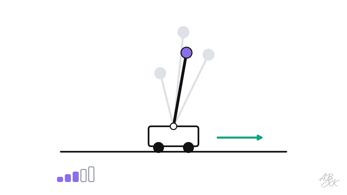
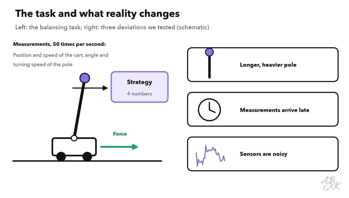
A cart can move left and right on a track, and a pole stands on it, held only by a hinge. Like balancing a broom on your hand, the cart has to move under the pole whenever it starts to fall. Fifty times per second, the strategy gets four measurements, the position and speed of the cart and the angle and turning speed of the pole, and decides how hard to push. An attempt counts as a success if the pole stays upright for ten seconds without the cart leaving the track.
| What changes | Fixed simulation | Random practice worlds |
|---|---|---|
| Mass of the cart | Always 1 kg | 0.5 to 2 kg |
| Mass of the pole | Always 0.1 kg | 0.05 to 0.4 kg |
| Length of the pole | Always the same | From a bit shorter to twice as long |
| Delay of the measurements | None | Up to 40 milliseconds |
| Sensor noise | None | From none to strong |
How the strategies learned
Both strategies are simple: four numbers that say how strongly to react to each measurement. They learned with the cross-entropy method: try 48 random strategies, keep the best eight, try new ones that resemble those, and repeat. After 25 rounds, both kept the pole upright for the full ten seconds in their own training worlds. In training, you could not tell them apart.
The test in the “real world”
The difference showed up in the test. As long as the test world matched the fixed simulation, both strategies succeeded in every attempt. A longer or heavier pole caused hardly any problems either. But when the measurements arrived 60 milliseconds late, the strategy from the fixed simulation succeeded in 0 of 100 attempts, the strategy from the random worlds in 100. With strong sensor noise, it was 57 against 100. In a random mix of all deviations, the closest thing to a real robot, the strategy from the fixed simulation succeeded in 51 of 100 worlds, the one from the random worlds in 97.
| Test condition | Trained in one fixed simulation | Trained with random variations |
|---|---|---|
| As in the simulation | 100 | 100 |
| Pole twice as long | 97 | 100 |
| Pole four times as heavy | 100 | 100 |
| Measurement 40 ms late | 20 | 100 |
| Measurement 60 ms late | 0 | 100 |
| Strong sensor noise | 57 | 100 |
| Random mix of all deviations | 51 | 97 |
Our own simulation: a pole on a cart (cart 1.0 kg, pole 0.1 kg, half length 0.5 m, force at most 10 N, step 0.02 s). Linear strategy, trained with the cross-entropy method (25 rounds, 48 candidates each); success = 10 s in balance. Random variations in training: cart 0.5–2.0 kg, pole 0.05–0.4 kg, half length 0.3–1.0 m, delay up to 2 steps, sensor noise. 100 attempts per test condition, fixed seed.
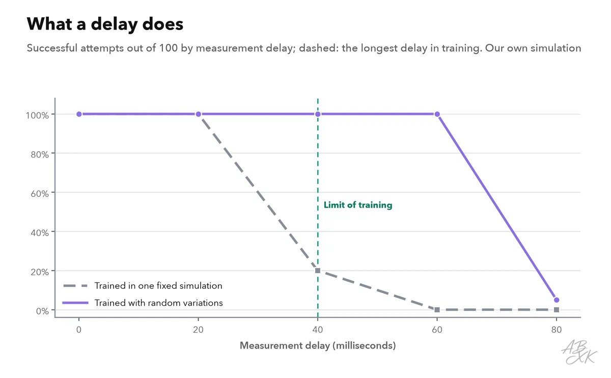
Why? The strategy from the fixed simulation learned to rely on perfect, instant measurements and reacts sharply. Each sharp reaction to a late measurement comes too late, and, as in the feedback loop of Level 1, the corrections start to swing. The strategy from the random worlds never had that luxury. It learned to react more calmly, which costs nothing when the world is perfect and saves it when the world is not.
The limits of randomization
The chart also shows the limit. At a delay of 80 milliseconds, twice as long as anything in the practice worlds, the strategy from the random worlds failed too. Randomization makes a strategy robust within the range it practiced, not beyond. It also has costs: training needs more attempts, and a strategy that has to work everywhere may be slower or more careful than one tuned for a single, well-known robot.
In practice, robot builders therefore combine several tools:
- Measuring the real robot to set the ranges of the simulation sensibly, for example by timing the real delays.
- Randomizing what matters, such as friction, masses, delays, lighting and camera positions for robots that see.
- Fine-tuning on the real robot with a small number of real attempts after the training in simulation.
- Learning from many robots at once, an idea behind the robot foundation models that this learning path covers in Level 0.
How we ran the experiment
We implemented the classic equations of the cart and pole in Python with numpy, with time steps of 20 milliseconds and a maximum force of 10 newtons. Each strategy is a linear rule with four numbers. Training ran for 25 rounds with 48 candidates of five attempts each. For every test condition, we ran 100 attempts with slightly different starting positions and a fixed random seed. The next part returns to the brain: what makes a decoder for brain signals better or worse.