

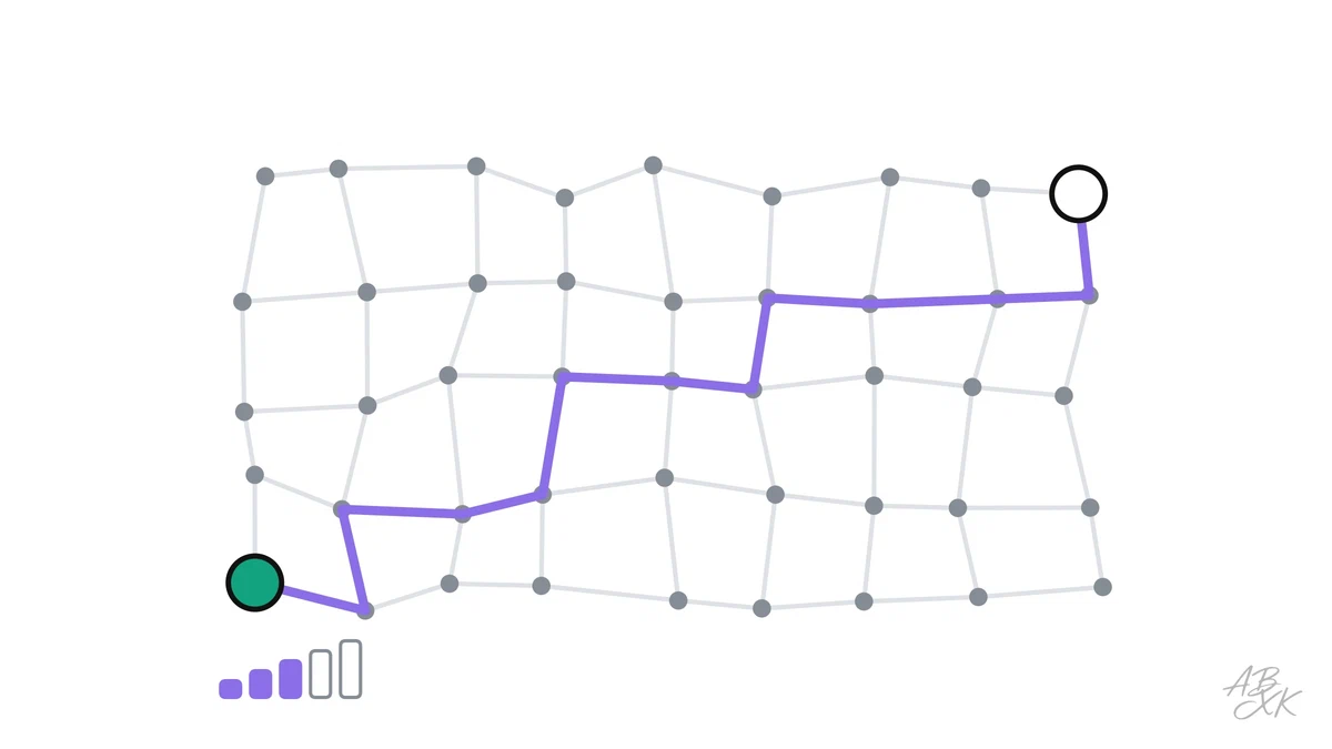
Once a machine has a map, it can plan. A navigation app, a delivery robot and a robotaxi all solve the same basic task thousands of times a day: find the shortest route from here to there through a network of streets or corridors. The task sounds simple, but a city has tens of thousands of intersections, and checking every possible route would take forever. The methods that solve it quickly are some of the oldest and most important algorithms in computing.
This is part 2 of Level 2 in our learning path Physical AI. We took the real street network of a part of San Francisco, a city where robotaxis are part of everyday traffic, from OpenStreetMap and planned 300 random routes with five different search methods. You will learn how a street map becomes a graph, how Dijkstra’s algorithm and A* search it and why the fastest methods do not always find the shortest route.
The street network as a graph
For a computer, a street map is a graph: intersections and bends are nodes, the road segments between them are edges, and each edge has a weight, here its length in meters. Our section of San Francisco, from Downtown to the Mission, contains 6,170 nodes that are all reachable from each other and 187 kilometers of road. 46.9% of the road segments can only be driven in one direction, which forces routes into detours that a pedestrian would not need.
| Term | What it means | In our map |
|---|---|---|
| Node | A point where the route can change | Intersections and bends |
| Edge | A connection between two nodes | A road segment between two intersections |
| Weight | The cost of using an edge | Length in meters |
| One-way edge | An edge in only one direction | Almost half of all segments |
| Estimate (heuristic) | A guess of the remaining cost | Straight-line distance to the goal |
Dijkstra: searching in every direction
Dijkstra’s algorithm, published in 1959, works like a wave spreading from the start. It always continues with the closest node it has not finished yet, so it reaches every node on the shortest possible way. When the wave reaches the goal, the route is guaranteed to be the shortest. The catch: the wave spreads in every direction, also away from the goal.
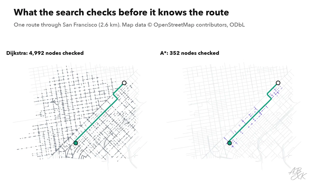
For our routes of 1 to 3 kilometers, Dijkstra checked 4,132 nodes in the median, about two thirds of the whole network. On the example route above, 2.60 kilometers long for a straight-line distance of 2.38 kilometers, it checked 4,992 nodes.
A*: a sense of direction
A* (pronounced “A star”) adds one piece of knowledge: an estimate of the remaining distance. We use the straight-line distance to the goal. A* always continues with the node where the distance so far plus the estimate is smallest, so the search leans toward the goal. As long as the estimate never overestimates the true remaining distance, and no street is shorter than the straight line, A* still finds the shortest route.
On our routes, A* checked 816 nodes in the median, 76.4% fewer than Dijkstra on average, and it found the shortest route every single time. On the example route, it needed only 352 nodes.
Faster, but no longer the shortest
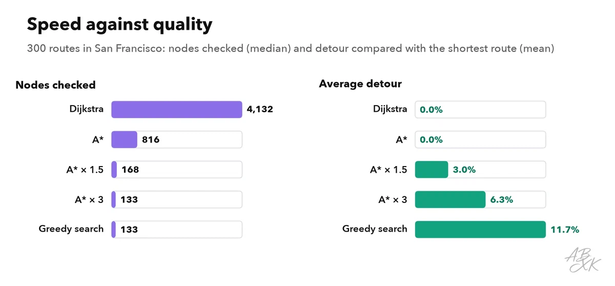
You can make A* even faster by trusting the estimate more. Weighted A* multiplies the estimate by a factor. With a factor of 3, the search checked only 133 nodes in the median, but it found the shortest route in only 12.3% of the cases, with an average detour of 6.3%. The extreme case is greedy best-first search, which only follows the estimate and ignores the distance already traveled. It was just as fast, 133 nodes in the median, but its routes were 11.7% longer on average and up to 67.9% longer: it heads straight for the goal and can run into one-way streets and dead ends that force long detours.
| Method | Nodes checked (median) | Shortest route found | Average detour | Largest detour |
|---|---|---|---|---|
| Dijkstra | 4,132 | 100.0% | 0.0% | 0.0% |
| A* (straight line as estimate) | 816 | 100.0% | 0.0% | 0.0% |
| Weighted A* (factor 1.5) | 168 | 16.7% | 3.0% | 25.0% |
| Weighted A* (factor 3) | 133 | 12.3% | 6.3% | 40.3% |
| Greedy best-first search | 133 | 7.7% | 11.7% | 67.9% |
Data: © OpenStreetMap contributors, license ODbL 1.0, retrieved on October 18, 2026; area of San Francisco (Downtown, SoMa, Mission), 6170 intersections and nodes, 187 km of road, one-way streets respected. Our analysis: 300 random routes with 1–3 km straight-line distance, fixed seed; we count the nodes the search completed.
What real systems add
Our experiment shows the core of route planning. Real systems build on it in several ways:
- Time instead of distance. Navigation weighs edges by expected travel time, with speed limits, traffic, waiting times at lights and the extra cost of left turns.
- Preparation in advance. Navigation services prepare their road networks so that routes across a whole continent can be answered in milliseconds; the search itself then checks only a few hundred nodes.
- Layers of planning. A robotaxi plans the route through the city first, then its behavior, such as when to change lanes, and finally the exact trajectory for the next few seconds, which the controller has to follow.
- Planning again. When a street is blocked or a robot meets an obstacle, the plan is recomputed, many times per minute if needed.
How we analyzed the data
We downloaded all drivable streets in a section of San Francisco from OpenStreetMap, respected one-way streets and kept only the part of the network in which every node can be reached from every other. We drew 300 random start and goal points with a straight-line distance of 1 to 3 kilometers, using a fixed random seed, and ran all five methods on every pair. We count the nodes a method has finished, a measure that does not depend on the speed of the computer. The next part follows a planned route on the road: how a self-driving car steers along it.