

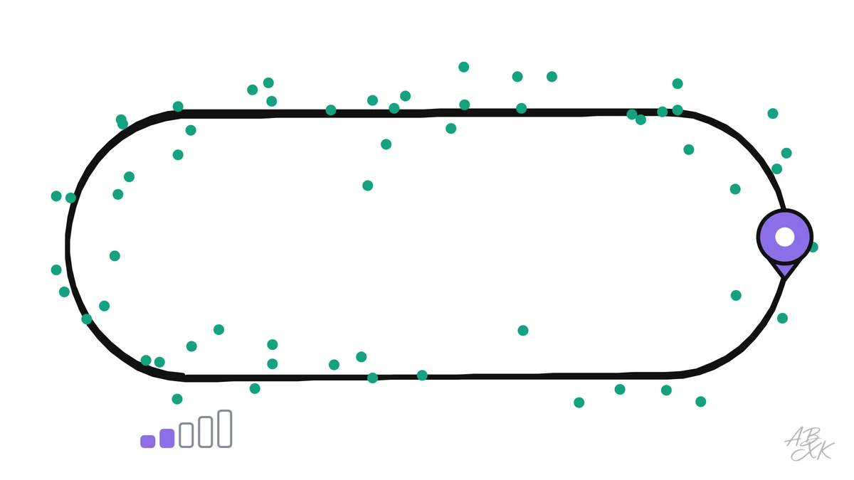
Before a robot can plan a path, it has to answer a simpler question: where am I? This task is called localization, and it is harder than it sounds. A delivery robot on a sidewalk, a vacuum robot in a living room and a self-driving car in a city all need to know their position, often to within a few centimeters, many times per second. No single sensor can deliver that on its own.
This is part 2 of Level 1 in our learning path Physical AI. We simulated a robot driving two laps of a track and compared three ways to track its position: counting wheel turns, GPS and a combination of both. You will learn why each sensor fails in its own way and how a Kalman filter combines them into something better than either.
Two kinds of position information
Robots get two kinds of information about where they are. Relative sensors measure movement: wheel encoders count how far the wheels turned, and a gyroscope measures how fast the robot turns. Adding up all the small movements is called odometry or dead reckoning. It is smooth and always available, but every small error is added to all the previous ones, so the estimate slowly drifts away.
Absolute sensors measure the position directly: satellite navigation (GPS), or a camera or lidar that recognizes known landmarks on a map. Their errors do not add up, but each single measurement can be off by meters, and they can fail completely, for example in a tunnel, in a parking garage or between tall buildings.
| Sensor | What it measures | Strength | Weakness |
|---|---|---|---|
| Wheel encoder | Distance traveled | Smooth, fast, cheap | Wheel slip and small scale errors add up |
| Gyroscope (IMU) | Rate of turning | Fast, works everywhere | A tiny drift turns into a large heading error |
| GPS | Position on Earth | No growing error | Meters of noise, fails in tunnels and indoors |
| Camera or lidar with a map | Position relative to known landmarks | Can be very precise | Needs a map made in advance and good visibility |
Our simulation: two laps, three methods
Our robot drives 428 meters in two laps of a stadium-shaped track, which takes 3.6 minutes. Its wheel sensor reads 2% too much, a typical small calibration error, and its gyroscope drifts by 0.1 degrees per second. GPS delivers a position once per second, scattered by about 3 meters, and fails completely for 30 seconds, as if the robot drove through a tunnel.
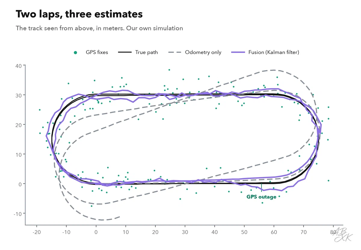
After one minute, odometry alone was only 1.4 meters off. By the end of the second lap, the error had grown to 14.2 meters, because the small errors in distance and heading kept adding up. GPS alone never drifted, but its single fixes were 3.7 meters off on average and up to 9.8 meters, too much to stay in a lane, and during the outage it gave no position at all.
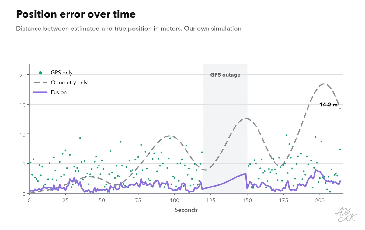
The combination was better than both. The fused estimate was off by 1.3 meters on average and never more than 4.2 meters. When GPS failed, the error grew from 0.7 to 3.3 meters, because the filter could only count wheel turns, and it dropped again as soon as the first satellite fixes came back.
| Method | Average error (m) | Largest error (m) | Error at the end (m) |
|---|---|---|---|
| Odometry only (wheels and gyroscope) | 6.8 | 14.2 | 14.2 |
| GPS only (single fixes) | 3.7 | 9.8 | – |
| Fusion in a Kalman filter | 1.3 | 4.2 | 2.0 |
Our own simulation: 2 laps of a stadium-shaped track (straights 60 m, curve radius 15 m, 2 m/s, 428 m in total). The wheel sensor reads 2% too much, the gyroscope drifts by 0.1 °/s; GPS once per second with 3 m spread, outage from second 120 to 150. Fusion: extended Kalman filter. Error = distance to the true position; fixed random seed.
How the Kalman filter combines the two
A Kalman filter works in two steps that repeat all the time. In the prediction step, it moves its estimate forward with the odometry and notes that its uncertainty has grown a little. In the correction step, a new GPS fix arrives, and the filter compares it with its prediction. It then moves the estimate toward the measurement, more strongly if its own uncertainty is high, less strongly if it trusts its prediction more than the noisy fix.
Think of walking through a familiar room with your eyes closed: you count your steps, and every few seconds you open your eyes for a moment. Between the glances, you rely on your steps; with each glance, you correct yourself. The filter does the same, but with numbers for how much it trusts each source. Our filter also estimated the heading, so the GPS fixes indirectly corrected the drifting gyroscope.
The same idea is behind nearly every positioning system in physical AI: phones combine GPS with motion sensors, drones combine satellite navigation with accelerometers, and self-driving cars combine many sensors at once.
Beyond GPS: maps and landmarks
For a self-driving car, an accuracy of a meter is not enough to stay in a lane. Many automated vehicles therefore also match what their lidar and cameras see against detailed maps made in advance: curbs, poles, lane markings and building edges. Such map matching can reach an accuracy of a few centimeters, but only where the map exists and is up to date. This is one reason why robotaxis operate in limited areas that their operators have mapped.
Robots that work indoors, where there is no GPS at all, often build the map while they move. This is called SLAM, simultaneous localization and mapping: the robot recognizes places it has seen before and uses them to correct its drift, just as GPS did in our simulation.
How we ran the simulation
We computed the robot’s movement in steps of 0.1 seconds in Python with numpy, with a fixed random seed for the sensor noise. The filter is an extended Kalman filter with three states: the two coordinates and the heading. The errors in the table are distances between estimated and true position; for GPS, we measured each single fix. The next part looks at the conditions under which self-driving cars operate and what US crash reports reveal about them.