
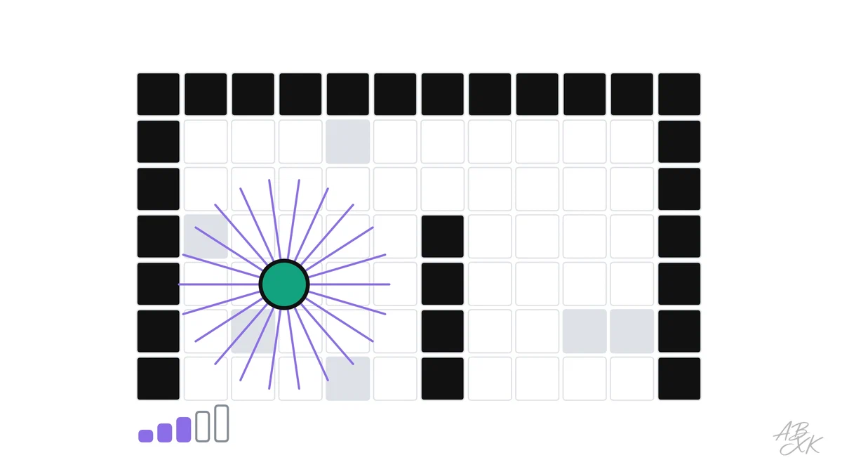
A robot that enters a new building knows nothing about it. Before it can plan a route to the loading dock or the kitchen, it has to find out where the walls, shelves and doors are. It builds this knowledge from what its sensors see, scan by scan, into a map. The most common kind of map for this is the occupancy grid: the floor is divided into small squares, and for each square the robot estimates whether it is free, occupied or still unknown.
This is part 1 of Level 2 in our learning path Physical AI, which looks at how the systems work inside. We simulated a robot with a lidar sensor driving through a made-up warehouse with four rooms, shelves and doors. You will learn what a lidar scan contains, how a grid map collects evidence from many scans and why the best map is worthless if the robot is wrong about its own position.
What a lidar sees
A 2D lidar is a laser that spins and measures the distance to the nearest object in many directions. Our simulated sensor sends 360 beams per turn, one per degree, with a range of 10 meters and a measurement noise of about 2 centimeters, typical values for the lidars on delivery and warehouse robots. Every beam tells the robot two things at once: the space along the beam up to the measured distance is free, and the point where the beam stopped is occupied. A beam that hits nothing within its range only says that the space along it is free.
Evidence instead of yes or no
The robot does not simply mark a square as free or occupied after one reading. Sensors make mistakes, people walk through the beam, and glass can reflect a laser in strange directions. Instead, every square keeps a running score, called log-odds. Each time a beam passes through the square, the score goes down a little; each time a beam ends in it, the score goes up. Only when enough evidence has collected does the square count as free or occupied. A single wrong reading changes the score, but it cannot overturn many good ones.
| State of a square | What it means | Typical cause |
|---|---|---|
| Unknown | No beam has reached it yet | Behind a wall, around a corner, out of range |
| Free | Many beams passed through it | Open floor, hallways, doorways |
| Occupied | Many beams ended in it | Walls, shelves, pillars |
| Unsure | Evidence points both ways | Moving people, glass, edges of objects |
Our simulation: the map grows with every scan
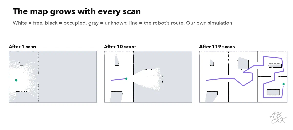
Our robot drove 55.6 meters through the building and took a scan every half meter, 119 scans in total. After ten scans, it had explored 42.4% of the free floor area, mostly the first room. By the end, it had explored 94.3%. The remaining patches lie behind shelves and in corners that no beam could reach from the robot’s route. Because the robot in this run knew its exact position, the walls in the map sit where they belong: 100% of the squares marked as occupied lie on or right next to a real wall.
| Scans | Area explored | Walls on target |
|---|---|---|
| 5 | 35.2% | 100.0% |
| 10 | 42.4% | 100.0% |
| 20 | 62.2% | 100.0% |
| 40 | 70.3% | 100.0% |
| 80 | 89.0% | 100.0% |
| 119 | 94.3% | 100.0% |
| 119, drifting position | 93.8% | 55.9% |
Our own simulation: a made-up floor plan of 24 × 14 m, grid 10 cm; lidar with 360 beams, range 10 m, noise 2 cm; one scan every 0.5 m along a 55.6 m route. Occupancy grid with log-odds. Drift: heading 0.1 °/m, distance 2% too long. Explored = share of the free area recognized as free; on target = share of cells marked occupied that lie at most one cell from a real wall.
The first scans add the most, and the curve then flattens. Every new room brings a jump, every turn into a known corridor adds little. This is why mapping robots plan their routes to visit places they have not seen yet, a strategy called exploration.
Why the position must be right
The map is only as good as the robot’s knowledge of where it stood for each scan. In a second run, we used exactly the same scans, but the robot placed them at the position it estimated from its wheels and gyroscope. As in our simulation of localization in Level 1, this estimate drifts slowly: here by 0.1 degrees of heading per meter and 2% in distance.
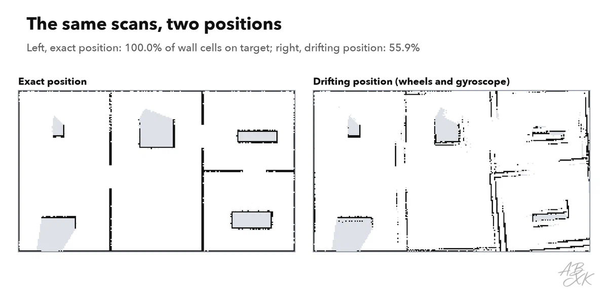
The result is a map in which walls appear twice, slightly rotated and shifted. Only 55.9% of the occupied squares still lie at a real wall; 44.1% are ghost walls that do not exist. A robot planning with this map would see closed doors where there are openings and open space where there is a shelf.
This is why mapping and localization are solved together. The method is called SLAM, simultaneous localization and mapping. While the robot builds the map, it also compares each new scan with the map so far and corrects its position when the two do not fit. When it returns to a place it has seen before, it can correct the drift of the whole loop at once, which is called loop closure.
What changes in the real world
Our simulation shows the core of the method, but real buildings are harder:
- Glass and mirrors. Lasers pass through glass doors or bounce off mirrors, so the map can show walls in the wrong place or none at all.
- Moving things. People, forklifts and doors change the scene. Robots keep their maps up to date and treat moving objects separately.
- Three dimensions. A 2D lidar at one height misses a table top or an overhanging shelf. Many robots therefore combine it with 3D lidar or depth cameras.
- Size and memory. A warehouse of several hectares at 10 centimeters per square needs millions of squares, so large maps are split into tiles and loaded as needed.
How we ran the simulation
We drew a floor plan of 24 by 14 meters with four rooms, five shelves and doors, divided it into squares of 10 centimeters and computed the lidar beams against the walls in Python with numpy, with a fixed random seed for the noise. Explored means the share of the free floor area that the map marks as free; on target means the share of occupied squares that lie at most one square from a real wall. The next part of this level uses a map to plan: how a robot or a car finds the shortest route through a real street network.