
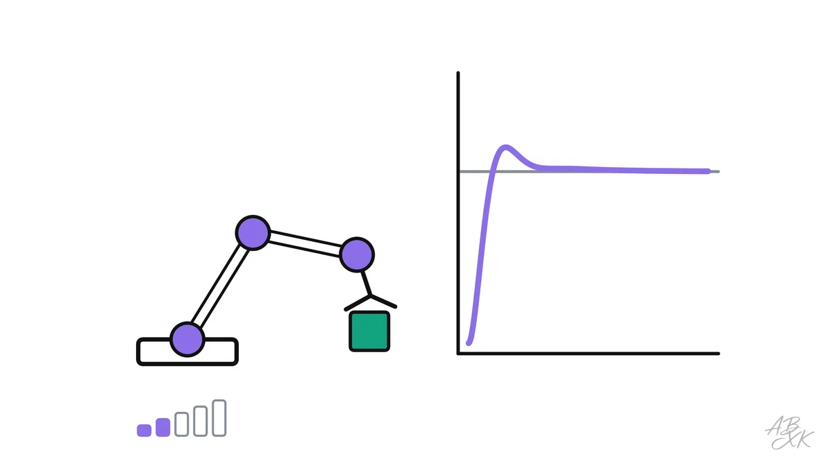
Every physical AI system ends in a motor. The AI decides “move the gripper 30 centimeters to the left” or “hold this lane at the current speed”, but something still has to make the motors do exactly that, against friction, heavy loads, wind and bumps in the road. That job belongs to feedback control, a field much older than modern AI. It is the layer that sits underneath every robot, drone and self-driving car.
This is part 1 of Level 1 in our learning path Physical AI. We simulated a simple robot joint and tested four classic controllers on it. You will learn what a control loop is, what the P, I and D in a PID controller do and why a delay of a fraction of a second can turn a calm machine into a shaking one.
The control loop
A controller works in a loop that never stops: it measures where the machine is, compares that with where it should be, computes a correction and sends it to the motor. Then it measures again. The difference between target and measurement is the error, and the whole art of control is to make the error small, quickly and without wild swings.
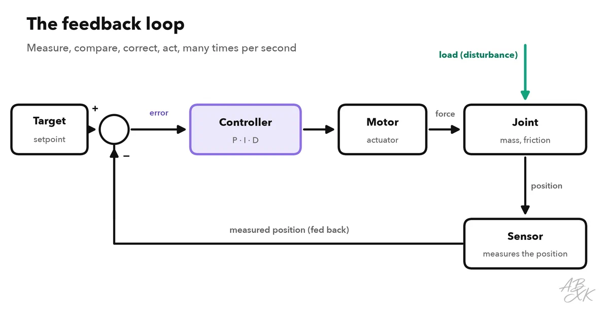
You use the same loop when you adjust the water in the shower: too cold, turn it up; too hot, turn it down. The shower also shows the main difficulty. The water needs a moment to reach you, and if you react to the old temperature, you overshoot.
| Term | What it means | In our simulation |
|---|---|---|
| Setpoint | Where the machine should be | Position 1 |
| Error | Setpoint minus measured value | Starts at 1, should end at 0 |
| Controller | Computes the force from the error | P, PI, PD or PID |
| Actuator | Turns the command into motion | A motor pushing the joint |
| Disturbance | Everything that pushes from outside | A constant load pulling against the motor |
Our simulation: one joint, four controllers
Our joint has a mass of 1 kilogram, some friction and a constant load of 3 newtons pulling against the motor, like a weight hanging from a robot arm. Its job is to move from position 0 to position 1 and stay there. We gave four controllers the same gains and the same task.
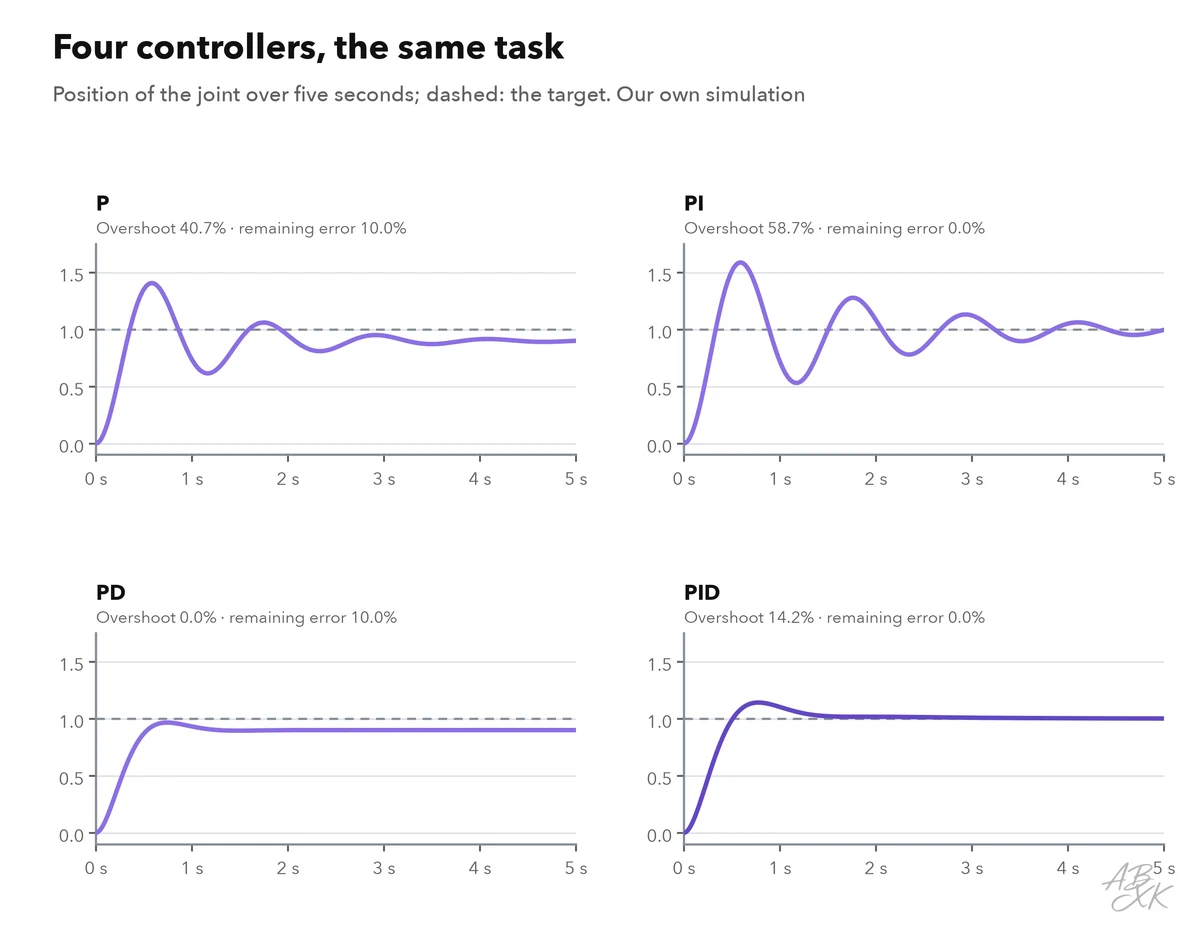
The P in PID stands for proportional: the bigger the error, the harder the motor pushes. Our P controller shot 40.7% past the target and then settled 10% short of it. The reason: to hold the load, a P controller needs a remaining error, because without an error it does not push at all.
The I stands for integral: the controller adds up the error over time and keeps pushing harder as long as any error is left. The PI controller removed the remaining error, but it overshot by 58.7% and needed 5.96 seconds to calm down. The D stands for derivative: it reacts to how fast the error changes and brakes early, like a driver who lifts off the gas before a red light. The PD controller did not overshoot at all, but it stopped 10% short, just like P.
Together, the three parts complement each other. Our PID controller reached the target with an overshoot of 14.2%, settled within 1.54 seconds and left no remaining error.
| Controller | Overshoot | Remaining error | Settling time (s) |
|---|---|---|---|
| P | 40.7% | 10.0% | 3.65 |
| PI | 58.7% | 0.0% | 5.96 |
| PD | 0.0% | 10.0% | 1.07 |
| PID | 14.2% | 0.0% | 1.54 |
Our own simulation: a joint with a mass of 1 kg and friction of 2 N·s/m moves against a constant load of 3 N to the target position 1; gains P = 30, I = 20, D = 5; time step 1 ms, 20 s simulated. Settling time: from then on, the position stays within ±2% of its final value.
Why a small delay is dangerous
A controller can only react to what it measures, and every measurement is a little late: sensors need time, data travels through cables and networks, software needs time to compute. We gave our PID controller the same task again, but with a delayed measurement.
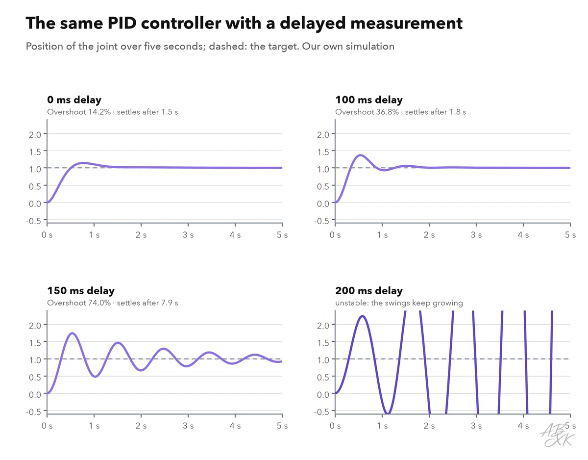
With a delay of 100 milliseconds, the overshoot rose to 36.8%. At 150 milliseconds, it was 74%, and the joint needed 7.9 seconds to settle. At 200 milliseconds, the joint never settled: the controller kept correcting a situation that was already over, and every swing grew larger than the one before. Engineers call this instability, and it is one of the most dangerous failures a machine can have.
| Delay (ms) | Overshoot | Settling time (s) | Result |
|---|---|---|---|
| 0 | 14.2% | 1.54 | settles |
| 50 | 19.6% | 2.01 | settles |
| 100 | 36.8% | 1.82 | settles |
| 150 | 74.0% | 7.90 | settles |
| 200 | – | – | oscillates more and more (unstable) |
Source as for the first table on this page.
The exact limit depends on the machine and the gains, but the pattern is general. That is why the fast control loops of robots and vehicles run close to the motors and repeat many times per second, while slower tasks, such as planning a route, can run on a computer further away. It is also why remote control of vehicles over a mobile network is hard: a delay that is harmless in a video call can be too much for a steering loop.
Where AI fits in
In most machines today, AI and classic control work in layers. AI handles the hard, open questions: what is in front of the camera, where the free space is, which path to take. Classic control then turns the planned path into motor commands, fast and reliably. Some newer robots, especially walking robots, use controllers trained with reinforcement learning in simulation instead of hand-tuned PID loops. But they face the same physics: delays, loads and limits of the motors. A learned controller that ignores them will shake just like our joint did.
Tuning a controller is always a trade-off. Higher gains make a machine faster but less calm; more damping makes it calm but slow. A controller that works well with one load can fail with another, so engineers test it under the worst conditions they expect.
How we ran the simulation
We wrote the simulation in Python with numpy and computed the motion in steps of one millisecond for 20 seconds. All controllers used the same gains, and the settling time is the moment from which the position stays within ±2% of its final value. Real machines also have motors with limited force, sensor noise and flexible parts, so the exact numbers will differ, but the effects of P, I, D and delay are the same. The next part of this level turns from motion to position: how a robot knows where it is.