

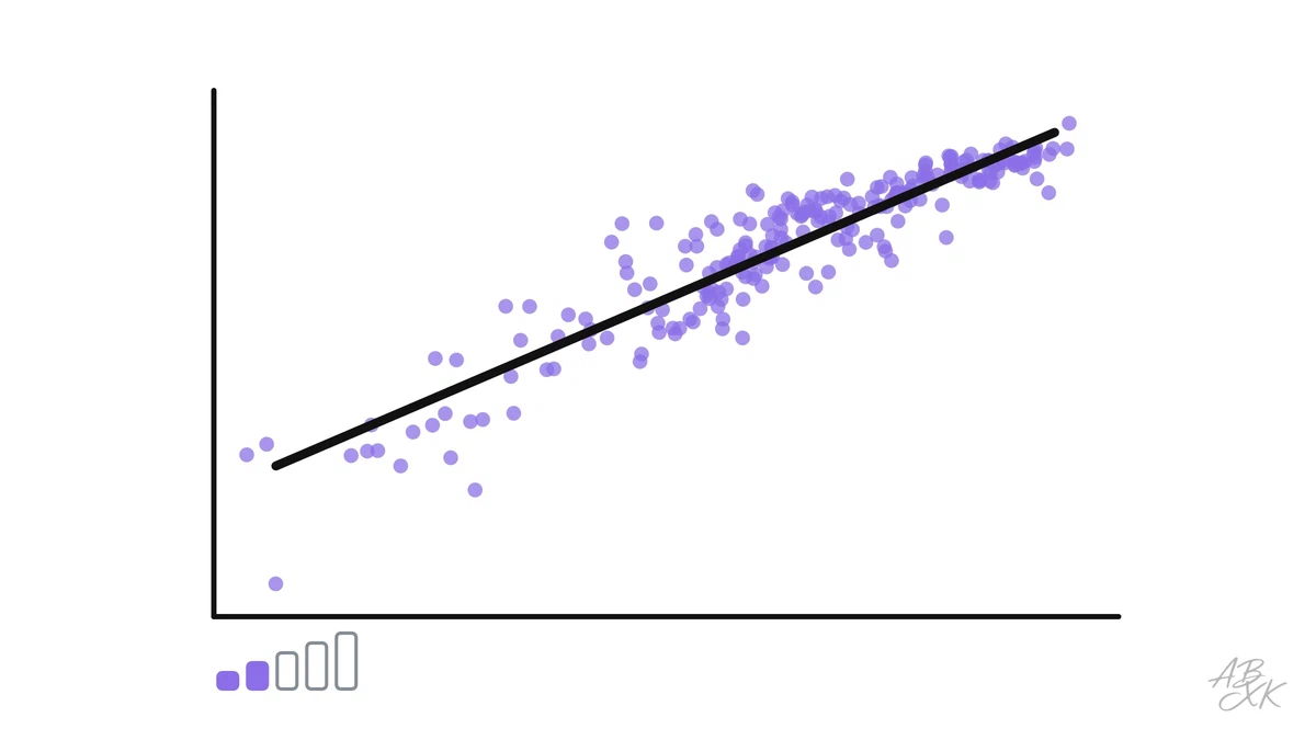
How many units will we sell next month? How long will this delivery take? What will this apartment cost? Whenever the answer is a number, the machine learning tool for the job is regression. It is the oldest method in this learning path, far older than computers, and it is still everywhere: in sales forecasts, in pricing, in the planning tools of almost every company.
This is part 1 of Level 1 in our learning path AI Fundamentals. Instead of the usual example with apartment prices, we use a question from the AI world itself: can you predict how much computing power the training of an AI model took from the number of its parameters? You will learn what a regression line is, how to read its slope, what R² tells you and why the points that miss the line are often the most interesting ones.
A line through the data
Epoch AI, a research institute that tracks the development of AI, records both the parameters and the training compute for 475 notable AI models. Both numbers span many orders of magnitude, from a few dozen parameters to trillions, so we plot them on logarithmic scales, where each step means ten times more. On these scales, the models line up surprisingly well.
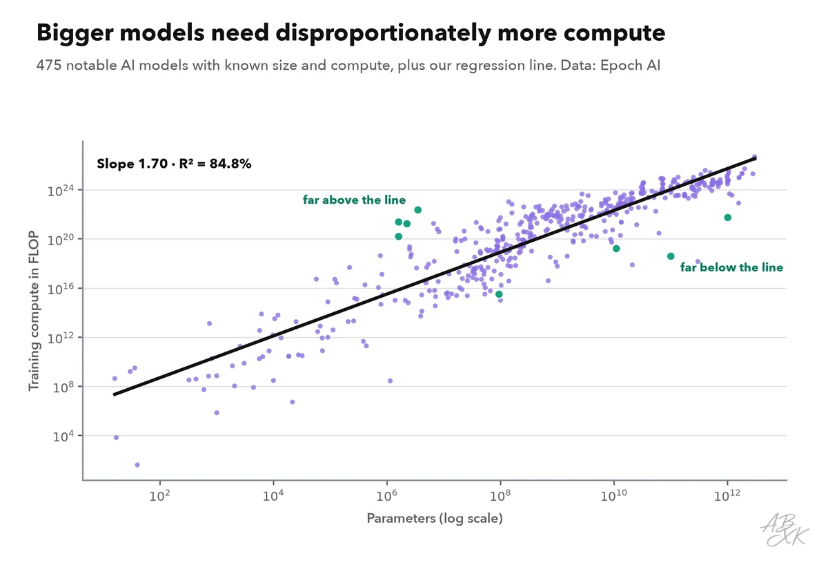
Linear regression draws the straight line that fits the points best. “Best” has a precise meaning: the line with the smallest sum of squared vertical distances to the points, called the least squares method. The line is described by two numbers. The intercept says where it starts; the slope says how steep it is. Our line has a slope of 1.70. On logarithmic scales that means: a model with ten times as many parameters needed, on average, about 50 times as much training compute. Bigger models do not just cost more to train, they cost disproportionately more, because they are usually also trained on more data.
| Term | What it means | In our example |
|---|---|---|
| Feature | The input the model uses | Number of parameters (log scale) |
| Target | The number to predict | Training compute (log scale) |
| Slope | How much the target changes per step of the feature | Ten times the parameters, about 50 times the compute |
| Intercept | Where the line crosses the axis | Compute of a hypothetical one-parameter model |
| Residual | Distance of a point from the line | How far a model is above or below the prediction |
| R² | Share of the variation the line explains | See below |
How good is the line?
The coefficient of determination, R², measures how much of the spread in the data the line explains: 0% means the line is useless, 100% means every point sits exactly on it. Our line explains 84.8% of the variation in training compute. That is high for real-world data. Still, a single prediction can be far off: on average, the actual compute differs from the line by a factor of about 17.4, up or down. Both statements are true at once. The line captures the big trend across many orders of magnitude; for one specific model, it is only a rough first guess.
The points that miss the line
Look at the residuals, the distances between the points and the line, and you learn what the model leaves out. Only 53.5% of the models lie within a factor of ten of the line, and 33 miss it by more than a factor of a thousand.
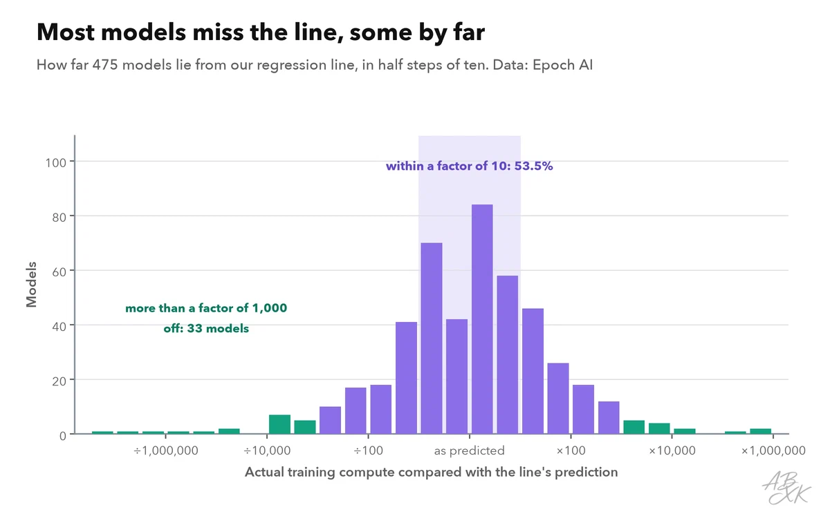
The models far above and far below our line are not random.
| Model | Organization | Year | Parameters | Actual compute compared with the line |
|---|---|---|---|---|
| GOAT | DeepMind | 2021 | 3.5 × 10⁶ | 891,251 times as much |
| StyleGAN3-R | Nvidia | 2021 | 1.6 × 10⁶ | 346,737 times as much |
| StyleGAN3-T | Nvidia | 2021 | 2.2 × 10⁶ | 134,896 times as much |
| IMPALA | DeepMind | 2018 | 1.6 × 10⁶ | 23,442 times as much |
| DLRM-2020 | Facebook AI | 2019 | 1.0 × 10¹¹ | 263,027 times less |
| M6-T | Alibaba | 2021 | 1.0 × 10¹² | 9,550 times less |
| ELMo | University of Washington | 2018 | 9.3 × 10⁷ | 2,239 times less |
| UnifiedQA | Allen Institute for AI | 2020 | 1.1 × 10¹⁰ | 1,479 times less |
Data: Epoch AI, Data on AI models (1078 notable models), retrieved on October 18, 2026, licensed CC BY 4.0; our analysis.
Far above the line are small networks that were trained for an unusually long time: agents that learned games and tasks through reinforcement learning, millions of rounds of trial and error, and image generators of the GAN type, which also train for many steps. Far below the line are models with huge numbers of parameters that are used only a little per example: a recommendation model whose parameters are mostly large lookup tables, and a mixture-of-experts language model in which only a small part of the network is active for each word. In both cases, the parameter count says little about the work done in training.
This is the second lesson of regression: a model is only as good as its features. Parameters alone explain a lot, but adding the amount of training data as a second feature would explain more, which is exactly what researchers do when they study how AI models scale.
Regression in practice
Regression is often the right first tool, even in projects that later move on to more complex models:
- Start simple. A linear regression trains in milliseconds, and its slope can be read and checked by anyone. More complex methods have to beat it to earn their place.
- Check the residuals. If the misses follow a pattern, for example always too low in winter, a feature is missing.
- Do not extrapolate far. A line fitted to the past says little about values far outside the data. Our line was fitted to models up to today’s largest; it cannot tell how much compute a model ten times larger would need.
- Correlation is not cause. The line shows that parameters and compute rise together, not that one causes the other. Both follow from the decision to build a bigger model.
How to measure the quality of a model that predicts a category instead of a number is the topic of the next part: classification and its metrics.