

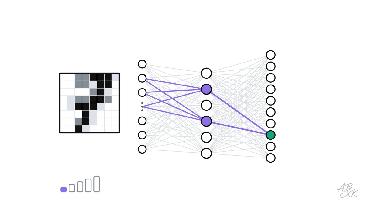
Neural networks are behind almost every recent AI breakthrough, from image recognition to large language models. The name sounds like biology, but the idea is simple arithmetic: many small calculations, connected in layers, with numbers that the network adjusts while it learns. To show what that means, we built and trained a small network ourselves and changed its size step by step.
This is part 5, the last part of Level 0 in our learning path AI Fundamentals. You will learn what a single artificial neuron computes, how neurons form layers, what the weights are and what happened to the accuracy of our network when we gave it more or fewer neurons.
One neuron: a weighted sum and a switch
An artificial neuron does two things. First, it multiplies each of its inputs by a weight and adds everything up, plus a constant called the bias. A large positive weight means “this input matters and pushes the result up”, a negative weight means “this input pushes it down”. Second, it passes the sum through an activation function, a simple rule such as “if the sum is negative, output zero, otherwise output the sum”. This switch-like step is what lets networks learn patterns that are not just straight lines.
That is all. One neuron is far too simple to recognize a digit. The power comes from connecting many of them.
Layers: from pixels to digits
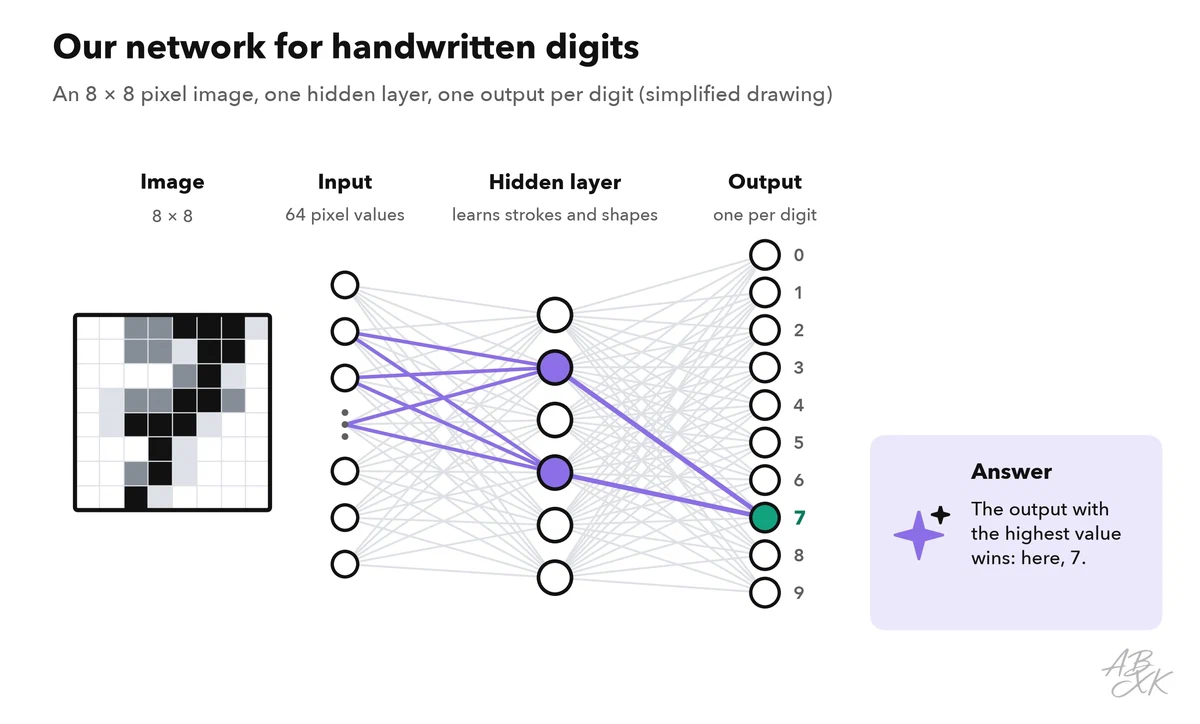
Our network reads the handwritten digits from part 2 of this level: images of 8 × 8 = 64 pixels. The input layer takes the 64 brightness values. A hidden layer of neurons combines them; each of its neurons is connected to all 64 inputs and learns to react to a certain stroke or shape. The output layer has 10 neurons, one per digit, and the one with the highest value is the network’s answer. “Hidden” only means that you never see these values directly; they are the network’s internal features.
Deep learning stacks many hidden layers. In image networks, the first layers react to edges, later ones to shapes and the last ones to whole objects, a hierarchy the network finds on its own during training.
Weights: what the network learns
Every connection has a weight, and every neuron a bias. Together they are the network’s parameters. Training, explained in part 3, adjusts them: the network predicts a digit, a formula measures how wrong it was, and an algorithm called backpropagation calculates how each weight should change to make the error smaller. Our network with 64 hidden neurons has 4,810 such numbers. A large language model has billions, but each one plays the same role.
| Part | What it is | In our network |
|---|---|---|
| Input layer | The raw data as numbers | 64 pixel brightness values |
| Hidden layer | Neurons that combine the inputs into features | Between 1 and 128 neurons |
| Output layer | One neuron per possible answer | 10 neurons, digits 0 to 9 |
| Weights and biases | The numbers adjusted in training | A few dozen to several thousand |
| Activation function | The switch inside each neuron | Negative sums become zero |
Our experiment: how many neurons does it take?
We trained the same network with 1, 2, 4, 8, 16, 32, 64 and 128 neurons in the hidden layer and tested each version on images it had never seen.
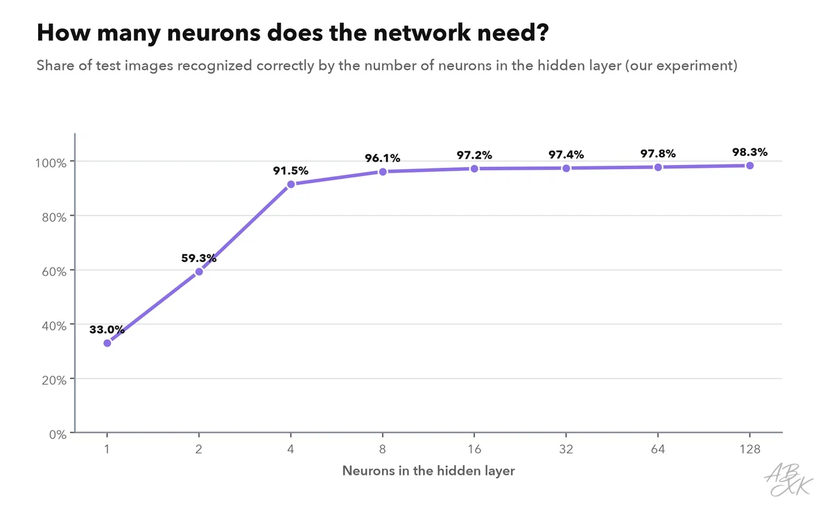
With a single hidden neuron, the network recognized only 33% of the digits: everything it knew had to squeeze through one number. With 8 neurons it already reached 96.1%, and with 64 neurons 97.8%. After that, more neurons barely helped. The lesson carries over to large models: size matters a lot until a network is big enough for its task and its data; beyond that, you need more or better data, not just more neurons.
| Neurons in the hidden layer | Weights and biases | Test images recognized correctly |
|---|---|---|
| 1 | 85 | 33.0% |
| 2 | 160 | 59.3% |
| 4 | 310 | 91.5% |
| 8 | 610 | 96.1% |
| 16 | 1,210 | 97.2% |
| 32 | 2,410 | 97.4% |
| 64 | 4,810 | 97.8% |
| 128 | 9,610 | 98.3% |
Our own experiment: dataset Optical Recognition of Handwritten Digits (E. Alpaydin, C. Kaynak, UCI Machine Learning Repository, license CC BY 4.0), 1797 images of 8 × 8 pixels, 540 of them held back for testing; scikit-learn 1.9.1, fixed random seed, so every run gives the same numbers.
A look inside our network
Each hidden neuron has one weight per pixel, so its 64 weights can be drawn as an 8 × 8 image. We did this for a version of our network with 16 hidden neurons, which recognized 97.2% of the test digits. Purple pixels push a neuron to fire, green pixels hold it back.
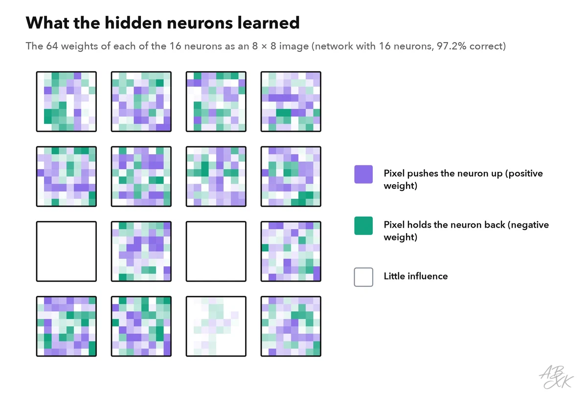
The images show two things that are typical of neural networks. First, no neuron looks like a clean digit. Each one reacts to a blurry mix of strokes, for example ink in the center and none at the edges, and only the combination of many neurons identifies a digit. Second, two of the 16 neurons stayed completely empty, and one more almost: their weights ended up near zero, so they never fire and do no work. Such unused or “dead” neurons are common, and they are one reason why networks are often built larger than they strictly need to be.
Why this matters for large models
A large language model is, at its core, the same thing at a gigantic scale: inputs turned into numbers, many layers of neurons, billions of weights adjusted in training, and an output layer that picks the next word piece. What makes it powerful is the architecture of its layers, the transformer, and the amount of data and compute behind it, which Level 3 and Level 4 of this learning path cover in detail.
Level 1 of this learning path turns to classic machine learning: regression, classification, clustering and how to tell whether a model is any good.