

Machine learning offers dozens of methods for the same task, and every one of them has fans. Which one is best? The honest answer is: it depends on the data, and you only find out by testing. Testing fairly, however, is harder than it looks, because a single test can make a method look better or worse than it is by chance.
This is part 4 of Level 1 in our learning path AI Fundamentals. We ran six classic methods on the same handwritten digits and compared them with cross-validation, the standard way to test fairly. You will learn what each method does in one sentence, how cross-validation works, which method won on our data and why that does not make it the best method in general.
Six methods in one sentence each
| Method | How it decides | Strength | Weakness |
|---|---|---|---|
| Logistic regression | Weighs every pixel and adds up the evidence for each digit | Fast, easy to inspect | Only straight boundaries between categories |
| k-nearest neighbors | Looks up the most similar training images and lets them vote | No training at all, strong when similar means same | Slow with large data, needs a good similarity measure |
| Decision tree | Asks a series of yes-or-no questions about pixels | Easy to explain | Overfits quickly |
| Random forest | Lets hundreds of slightly different trees vote | Robust, little tuning needed | Harder to explain than one tree |
| Support vector machine | Draws the widest possible border between categories | Strong on medium-sized data | Slow on large data, many settings |
| Neural network | Learns its own features in a hidden layer | Most flexible | Needs more data and tuning |
Cross-validation: five tests instead of one
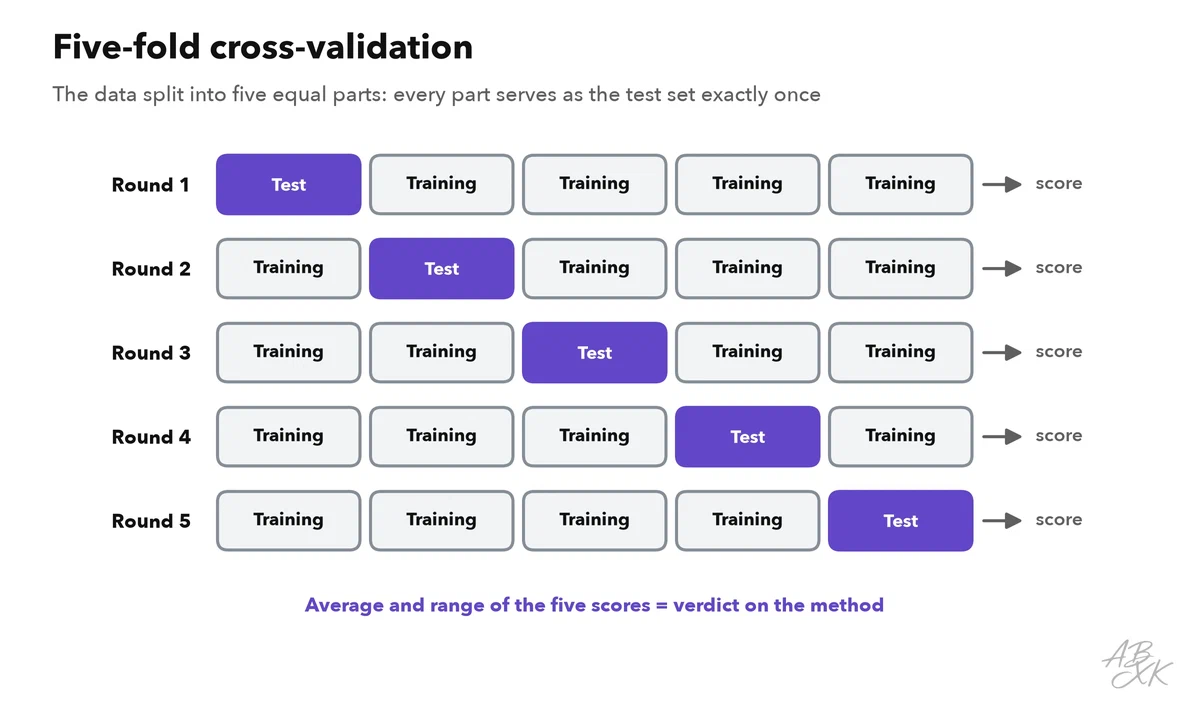
A single split into training and test data is a bit like a single exam: the result depends partly on which questions happened to come up. Cross-validation repeats the test. In five-fold cross-validation, the data is split into five equal parts. Each method is trained five times, each time on four parts, and tested on the fifth, so that every image is used for testing exactly once. The result is an average and a range, which shows how stable a method is.
The result on our data
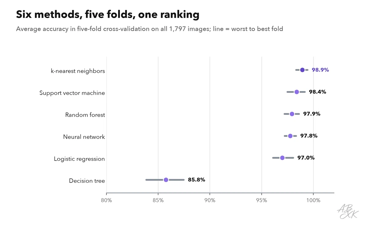
On the handwritten digits, the winner was k-nearest neighbors, with 98.9% on average, ahead of the support vector machine, the random forest and the neural network, which were close together. Logistic regression reached 97%. The single decision tree came last with 85.8%, and its results varied most between the folds, with a standard deviation of 1.6 percentage points.
| Method | Mean | Worst fold | Best fold |
|---|---|---|---|
| k-nearest neighbors (k = 3) | 98.9% | 98.3% | 99.4% |
| Support vector machine | 98.4% | 97.5% | 99.2% |
| Random forest (200 trees) | 97.9% | 97.2% | 98.6% |
| Neural network (64 neurons) | 97.8% | 97.2% | 98.3% |
| Logistic regression | 97.0% | 96.1% | 98.1% |
| Decision tree | 85.8% | 83.8% | 87.5% |
Our own experiment: dataset Optical Recognition of Handwritten Digits (E. Alpaydin, C. Kaynak, UCI Machine Learning Repository, license CC BY 4.0), 1797 images of 8 × 8 pixels, 540 of them held back for testing; scikit-learn 1.9.1, fixed random seed, so every run gives the same numbers.
Why does the simplest method win here? Because on these small, centered images, two handwritten 3s really do look alike pixel by pixel, so “find the most similar known example” works very well. On data where similarity is not so obvious, such as customer records with dozens of columns in different units, k-nearest neighbors usually falls behind, and tree ensembles or gradient boosting tend to lead.
Accuracy is not the whole bill
Two methods with almost the same accuracy can differ by orders of magnitude in what they cost to run. For each trained model, we counted what it has to keep in memory and how much work it does, at most, for every new image.
| Method | Keeps after training | Size | Work per new image (at most) |
|---|---|---|---|
| Logistic regression | Weights | 650 | 640 multiplications |
| k-nearest neighbors (k = 3) | All training images | 1,257 images, 80,448 pixel values | Compare with 1,257 images (80,448 pixel values) |
| Decision tree | Questions and leaves | 241 nodes | 11 questions |
| Random forest (200 trees) | Questions and leaves of all trees | 61,848 nodes | 2,653 questions |
| Support vector machine | Support vectors: training images near the borders | 686 images, 43,904 pixel values | Compare with 686 images (43,904 pixel values) |
| Neural network (64 neurons) | Weights and biases | 4,810 | 4,736 multiplications |
Source as for the first table on this page.
The winner on accuracy is the most expensive to run. k-nearest neighbors keeps all 1,257 training images, 80,448 pixel values, and compares every new image with each of them. Logistic regression gets by with 650 weights, about 124 times fewer numbers, and reached 97% in cross-validation instead of 98.9%. The support vector machine keeps only the training images close to the borders between digits, 686 of them. The neural network stores 4,810 weights, and the random forest 61,848 questions and leaves across its 200 trees.
With small images like ours, all of this fits easily on any phone. With millions of large images or documents, the difference decides whether a method can run at all. That is why k-nearest neighbors in production relies on special search indexes that find similar items without comparing against every single one, the same technology that vector databases are built on.
There is no best method
Machine learning research has a name for this observation: the no free lunch principle. No method is best for every kind of data. That is why practitioners follow a few habits:
- Start with a simple baseline, such as logistic regression. Every more complex method has to beat it clearly.
- Compare with cross-validation, not with one lucky split, and look at the range as well as the average.
- Count more than accuracy. Speed, memory, the cost of training and whether people can follow the decisions matter in production.
- Prefer the simpler model when results are close. A difference of a few tenths of a percent is often within the range of chance.
- Test on your own data. Benchmarks from other people’s data, including ours, only tell you what to try first.
How we ran the experiment
We used the Python library scikit-learn with mostly standard settings: k-nearest neighbors with k = 3, a random forest with 200 trees, a support vector machine with its standard kernel on standardized pixel values and a neural network with one hidden layer of 64 neurons. The five folds are stratified, so every fold contains about the same share of each digit, and the split uses a fixed seed, so the numbers on this page come out the same on every run. The counts in the cost table come from the models trained on the 1,257 training images. The last part of Level 1 turns to data without any labels: finding groups with clustering and simplifying data with PCA.