

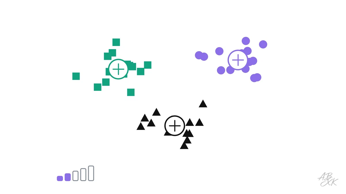
Most data in a company has no labels. Nobody has marked which customers belong together, which machine readings are normal or which documents cover the same topic. Unsupervised learning works with exactly this kind of data. It does not learn to predict a known answer; it looks for structure: groups of similar items, or a simpler way to describe the data.
This is part 5 of Level 1 in our learning path AI Fundamentals. We return to the handwritten digits, this time without telling the methods which digit each image shows. You will learn how k-means clustering finds groups, why the hardest question is how many groups to look for, and how principal component analysis (PCA) compresses each image from 64 numbers to a handful, plus what that does to the groups.
How k-means finds groups
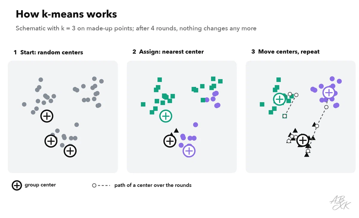
k-means needs one setting from you: the number of groups, called k. Then it repeats two simple steps:
- Assign. Every data point joins the group whose center is closest.
- Update. Every group center moves to the average of its members.
At the start, the centers are placed at random. After a few rounds, the assignments stop changing, and the method is done. Because the result depends on the random start, it is usually run several times, and the best run is kept. We used ten runs.
Our experiment: ten groups, no labels
We asked k-means for ten groups of the 1,797 digit images, without the labels. Afterward, we used the labels only to check what each group contains.
| Most common digit in the group | Images in the group | Share of that digit | Next most common digits (images) |
|---|---|---|---|
| 0 | 179 | 98.9% | 2 (1), 6 (1) |
| 4 | 168 | 98.8% | 0 (1), 5 (1) |
| 6 | 182 | 97.3% | 1 (2), 8 (2) |
| 5 | 157 | 87.3% | 8 (6), 9 (6) |
| 7 | 198 | 85.9% | 4 (8), 3 (7) |
| 3 | 181 | 85.6% | 2 (13), 9 (6) |
| 2 | 176 | 84.1% | 1 (24), 8 (3) |
| 1 | 89 | 61.8% | 9 (20), 8 (6) |
| 9 | 241 | 57.7% | 8 (48), 5 (41) |
| 8 | 226 | 45.1% | 1 (99), 2 (8) |
Our own experiment: dataset Optical Recognition of Handwritten Digits (E. Alpaydin, C. Kaynak, UCI Machine Learning Repository, license CC BY 4.0), 1797 images of 8 × 8 pixels, 540 of them held back for testing; scikit-learn 1.9.1, fixed random seed, so every run gives the same numbers.
Some groups are almost pure. The group that mostly contains zeros is 98.9% zeros, because a zero looks like nothing else. Other groups are mixed: in the group where 8 is the most common digit, only 45.1% of the 226 images are actually 8s. Almost all of the others, 99 images, are 1s: by the method’s measure of distance, many 1s are closer to the average 8 than to the average 1. The 1s end up split across several groups. Overall, 79.4% of the images land in the group of their own digit. That is impressive for a method that never saw a single label, and it is also a warning: groups found by an algorithm are similar by its measure of distance, not necessarily by the meaning you care about.
How many groups? The methods disagree
With the digits, we know the right answer: ten. With real business data, nobody does. Two common methods are supposed to help.
The elbow method runs k-means for many values of k and plots how far the points are from their group centers, in total. More groups always reduce this distance, so you look for the “elbow”, the point where adding groups stops paying off. The silhouette score checks for every point whether it is much closer to its own group than to the next one; a higher average score means cleaner groups.
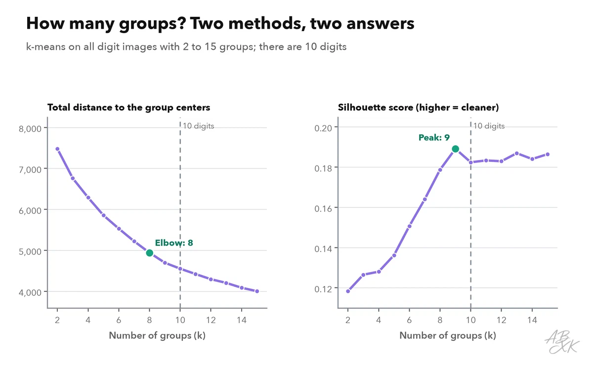
On our data, the elbow method pointed to 8 groups and the silhouette score to 9. Neither found the true ten. The curve bends only gently, and the best silhouette score, 0.19 on a scale from −1 to 1, is low, which means that the groups overlap a lot. This is typical for real data. The methods give you a range to try, but the final number of groups is a decision you make based on what the groups are for: five customer segments that a sales team can work with may be more useful than the twelve that score slightly better.
PCA: the same images in fewer numbers
Each digit image consists of 64 numbers, one per pixel. But the pixels are not independent: if the middle of a 0 is empty, its neighbors are probably empty too. Principal component analysis (PCA) uses this. It finds new directions in the data, called principal components, ordered by how much of the variation between the images they capture. The first direction captures the most, the second the most of what is left, and so on. Keeping only the first few directions describes each image with fewer numbers while losing as little as possible.
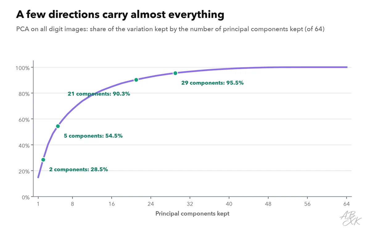
The curve rises steeply at first. Just 5 directions keep 54.5% of the variation, 21 keep more than 90%, and 29 keep more than 95%. The last directions add almost nothing: each of them describes a single pixel at the left or right edge of the image, and those pixels are nearly always empty.
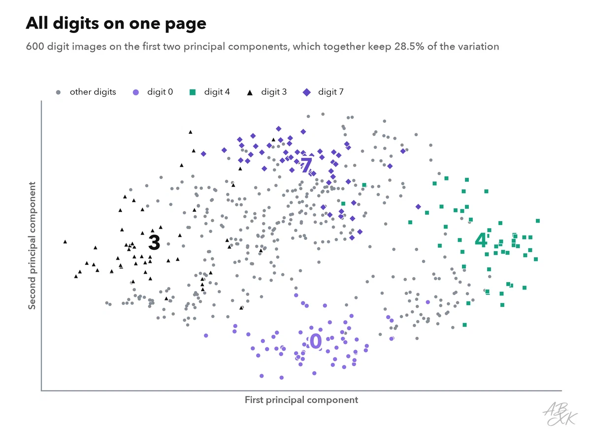
The first two directions alone keep only 28.5% of the variation, but they are enough to draw the whole dataset on a flat page. In this map, some digits form clear islands: zeros at the bottom, fours on the right, threes on the left and sevens at the top. Others overlap in the middle, among them the 1s, 8s and 9s, the digits that k-means mixed up most.
Compress first, then cluster
Fewer numbers per image make every later step faster and cheaper. But do the groups suffer? We ran k-means again after compressing the images with PCA.
| Directions kept (of 64) | Variation kept | k-means: images in the group of their digit |
|---|---|---|
| 2 | 28.5% | 59.4% |
| 5 | 54.5% | 71.7% |
| 13 | 80.3% | 78.7% |
| 21 | 90.3% | 79.6% |
| 64 | 100.0% | 79.4% |
Source as for the first table on this page.
With only two directions, k-means put just 59.4% of the images in the group of their digit, because too much information was lost. With 21 directions, the result was 79.6%, as good as with all 64 pixels (79.4%), with a third of the numbers. The directions that compression dropped carried little that mattered for the groups. This is why PCA and related methods are a standard first step before clustering, search and visualization. The embeddings that AI systems use to compare texts and images follow a related idea: they describe each item with a list of numbers in which similar items end up close together.
| Question | Clustering | PCA |
|---|---|---|
| What does it do? | Puts similar items into groups | Describes items with fewer numbers |
| What do you choose? | The number of groups | The number of directions to keep |
| Typical uses | Customer segments, grouping documents, spotting unusual cases | Charts of complex data, faster training, removing noise |
| Main risk | Groups that are similar by distance but not by meaning | Throwing away a small detail that matters |
How we ran the experiment
We used the Python library scikit-learn and its copy of the digit dataset, with all 1,797 images and pixel values scaled from 0 to 1. k-means ran ten times from different random starts for every number of groups, and the best run was kept. To find the elbow automatically, we took the point with the largest distance below a straight line from the first to the last point of the curve. The labels were used only to evaluate the groups, never to form them. All random choices use a fixed seed, so the numbers on this page come out the same on every run. Level 2 of this learning path turns to deep learning: what changes when networks get many layers.